PySATL Core: Usage Example

This notebook demonstrates the core capabilities of PySATL Core:

1. Registering built-in distribution families in the global registry.

2. Retrieving a family object from the registry and instantiating concrete distributions.

3. Querying and visualizing characteristics (PDF / CDF / PPF).

4. Sampling via inverse transform sampling.

5. Defining and registering a custom family with multiple parametrizations.

6. Using the characteristic graph to obtain missing characteristics.

Environment notes:

• Python 3.12+ is required.

• A family is an object stored in the singleton ParametricFamilyRegister.

Setup

PySATL provides configuration entry points that create family objects and register them:

• configure_normal_family() registers only the Normal family.

• configure_families_register() registers all built-in families shipped with the library.

You can access the registry without filling it by instantiating ParametricFamilyRegister().

import matplotlib.pyplot as plt
import numpy as np

from pysatl_core import (
    CharacteristicName,
    ContinuousSupport,
    FamilyName,
    ParametricFamily,
    ParametricFamilyRegister,
    Parametrization,
    UnivariateContinuous,
    configure_families_register,
    configure_normal_family,
    parametrization,
)

# Access the registry without configuring it
registry = ParametricFamilyRegister()
registry.list_registered_families()

[]

# Option A: register ONLY the Normal family
configure_normal_family()
registry.list_registered_families()

[<FamilyName.NORMAL: 'Normal'>]

# Option B: register ALL built-in families
configure_families_register()
registry.list_registered_families()

[<FamilyName.NORMAL: 'Normal'>,
 <FamilyName.EXPONENTIAL: 'Exponential'>,
 <FamilyName.CONTINUOUS_UNIFORM: 'ContinuousUniform'>]

1) Built-in family: Normal

A concrete distribution is obtained by fixing the parameters.

You can create it via:

• family(...) (uses the base parametrization by default), or

• family.distribution(parametrization_name=..., **params).

The Normal family ships with multiple parametrizations:

• meanStd (base): (mu, sigma)

• meanPrec: (mu, tau) where tau = 1 / sigma^2

• exponential: (a, b) (an exponential-family form)

normal_family = ParametricFamilyRegister.get(FamilyName.NORMAL)
normal_family.name, normal_family.parametrization_names

(<FamilyName.NORMAL: 'Normal'>, ['meanStd', 'meanPrec', 'exponential'])

Instantiating distributions in different parametrizations

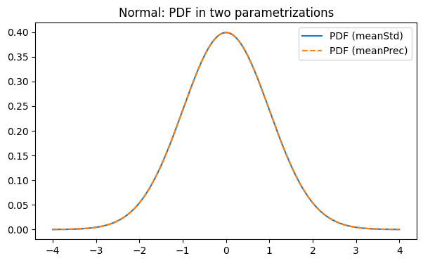
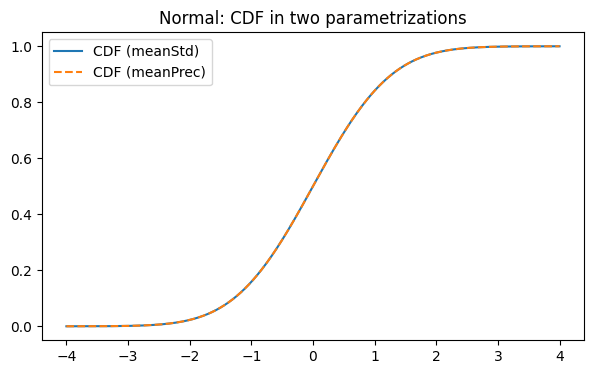
Below we instantiate the same distribution in two parametrizations:

• meanStd: parameters (mu, sigma)

• meanPrec: parameters (mu, tau) where tau = 1 / sigma^2

We then compare their PDF and CDF curves (they should match). Actually, all the characteristics are computed via base parametrization (meanStd). Other parametrizations are being transformed to base while computing

d_mean_std = normal_family.distribution(parametrization_name="meanStd", mu=0.0, sigma=1.0)
d_mean_prec = normal_family.distribution(parametrization_name="meanPrec", mu=0.0, tau=1.0)
d_mean_std.parametrization_name, d_mean_prec.parametrization_name

('meanStd', 'meanPrec')

x = np.linspace(-4, 4, 600)

pdf_std = d_mean_std.query_method(CharacteristicName.PDF)
cdf_std = d_mean_std.query_method(CharacteristicName.CDF)

pdf_prec = d_mean_prec.query_method(CharacteristicName.PDF)
cdf_prec = d_mean_prec.query_method(CharacteristicName.CDF)

plt.figure(figsize=(7, 4))
plt.plot(x, pdf_std(x), label="PDF (meanStd)")
plt.plot(x, pdf_prec(x), linestyle="--", label="PDF (meanPrec)")
plt.legend()
plt.title("Normal: PDF in two parametrizations")
plt.show()

plt.figure(figsize=(7, 4))
plt.plot(x, cdf_std(x), label="CDF (meanStd)")
plt.plot(x, cdf_prec(x), linestyle="--", label="CDF (meanPrec)")
plt.legend()
plt.title("Normal: CDF in two parametrizations")
plt.show()

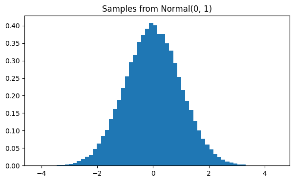
Sampling

For the Normal distribution, sampling is provided via the high-level distribution.sample(...) interface.

Internally, the sampling strategy may rely on analytical characteristics (such as PPF for inverse transform sampling), but this detail is hidden from the user. The recommended way to generate samples is always through sample(...), which ensures a consistent and efficient implementation.

At the moment, this only works with characteristics with NumPy semantics (so not graph computed).

samples = d_mean_std.sample(n=100_000)

plt.figure(figsize=(7, 4))
plt.hist(samples, bins=60, density=True)
plt.title("Samples from Normal(0, 1)")
plt.show()

2) Custom family with multiple parametrizations

In this section we create a custom family and register it in ParametricFamilyRegister.

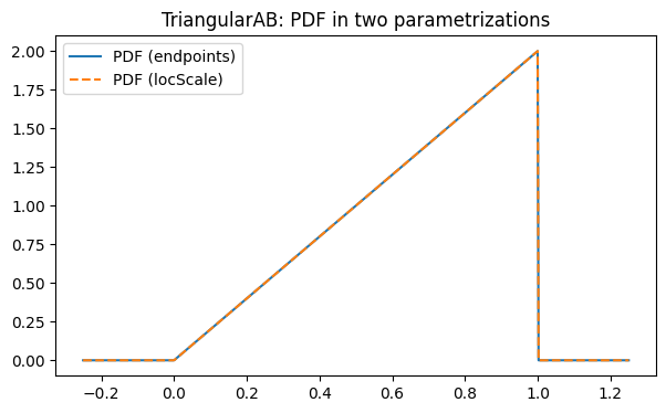
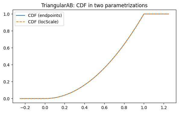
We implement a simple distribution on an interval [a, b] with CDF F(x) = ((x-a)/(b-a))^2 for x ∈ [a, b] (and 0/1 outside), which corresponds to the PDF f(x) = 2(x-a)/(b-a)^2 on [a, b].

We provide PDF and CDF analytically for both parametrizations, but omit PPF. Then we query PPF via the characteristic graph.

Parametrizations:

• endpoints: (a, b)

• locScale: (loc, scale) where a = loc, b = loc + scale

Important note (current limitation).

Built-in families provide analytical characteristics that follow NumPy semantics (arrays in / arrays out). Graph-based conversions (fitted methods from fitters.py) are currently scalar-only.

That means that a derived characteristic like PPF may only accept Python floats. If you pass a NumPy array, SciPy routines used inside conversions (e.g. scipy.integrate.quad) may fail with errors such as ValueError: The truth value of an array with more than one element is ambiguous.

Until the fitters are upgraded to NumPy semantics, evaluate derived characteristics pointwise.

def _ab(params: Parametrization) -> tuple[float, float]:
    if hasattr(params, "a") and hasattr(params, "b"):
        return float(params.a), float(params.b)
    return float(params.loc), float(params.loc + params.scale)


def tri_pdf(params: Parametrization, x: np.ndarray) -> np.ndarray:
    a, b = _ab(params)
    x = np.asarray(x, dtype=np.float64)
    denom = b - a
    y = 2.0 * (x - a) / (denom * denom)
    y[(x < a) | (x > b)] = 0.0
    return y


def tri_cdf(params: Parametrization, x: np.ndarray) -> np.ndarray:
    a, b = _ab(params)
    x = np.asarray(x, dtype=np.float64)
    denom = b - a
    t = (x - a) / denom
    return np.where(x <= a, 0.0, np.where(x >= b, 1.0, t * t))


def tri_support(params: Parametrization) -> ContinuousSupport:
    a, b = _ab(params)
    return ContinuousSupport(a, b)

tri_family = ParametricFamily(
    name="TriangularAB",
    distr_type=UnivariateContinuous,
    distr_parametrizations=["endpoints", "locScale"],
    distr_characteristics={
        CharacteristicName.PDF: {
            "endpoints": tri_pdf,
            "locScale": tri_pdf,
        },
        CharacteristicName.CDF: {
            "endpoints": tri_cdf,
            "locScale": tri_cdf,
        },
        # PPF intentionally omitted: it will be derived by the graph.
    },
    support_by_parametrization=tri_support,
)


@parametrization(family=tri_family, name="endpoints")
class Endpoints(Parametrization):
    a: float
    b: float


@tri_family.parametrization(name="locScale")
class LocScale(Parametrization):
    loc: float
    scale: float


# Register the family so that the computation strategy can resolve it by name
ParametricFamilyRegister.register(tri_family)
ParametricFamilyRegister.get("TriangularAB").name

'TriangularAB'

tri_endpoints = tri_family.distribution(parametrization_name="endpoints", a=0.0, b=1.0)
tri_locscale = tri_family.distribution(parametrization_name="locScale", loc=0.0, scale=1.0)
tri_endpoints.parametrization_name, tri_locscale.parametrization_name

('endpoints', 'locScale')

x01 = np.linspace(-0.25, 1.25, 600)

pdf_e = tri_endpoints.query_method(CharacteristicName.PDF)
cdf_e = tri_endpoints.query_method(CharacteristicName.CDF)
pdf_l = tri_locscale.query_method(CharacteristicName.PDF)
cdf_l = tri_locscale.query_method(CharacteristicName.CDF)

plt.figure(figsize=(7, 4))
plt.plot(x01, pdf_e(x01), label="PDF (endpoints)")
plt.plot(x01, pdf_l(x01), linestyle="--", label="PDF (locScale)")
plt.legend()
plt.title("TriangularAB: PDF in two parametrizations")
plt.show()

plt.figure(figsize=(7, 4))
plt.plot(x01, cdf_e(x01), label="CDF (endpoints)")
plt.plot(x01, cdf_l(x01), linestyle="--", label="CDF (locScale)")
plt.legend()
plt.title("TriangularAB: CDF in two parametrizations")
plt.show()

def eval_scalar_method_on_array(method, xs):
    xs = np.asarray(xs, dtype=np.float64)
    return np.array([method(float(x)) for x in xs], dtype=np.float64)

Querying a derived PPF (scalar-only)

We now request PPF. Since we did not provide it analytically, it is derived via the characteristic graph. At the moment, this derived method is scalar-only, so we evaluate it pointwise for a vector of probabilities.

ppf_e = tri_endpoints.query_method(CharacteristicName.PPF)
ppf_l = tri_locscale.query_method(CharacteristicName.PPF)

qs = np.array([0.1, 0.25, 0.5, 0.75, 0.9])
q_endpoints = np.array([ppf_e(float(q)) for q in qs], dtype=np.float64)
q_locscale = np.array([ppf_l(float(q)) for q in qs], dtype=np.float64)
np.column_stack([qs, q_endpoints, q_locscale])

array([[0.1       , 0.31622777, 0.31622777],
       [0.25      , 0.5       , 0.5       ],
       [0.5       , 0.70710678, 0.70710678],
       [0.75      , 0.8660254 , 0.8660254 ],
       [0.9       , 0.9486833 , 0.9486833 ]])

Summary

• Built-in families: analytical methods support NumPy arrays.

• Custom family: we registered it in the global registry.

• We provided vectorized PDF and CDF.

• We omitted PPF, and obtained it via the characteristic graph.

• Graph-derived methods are currently scalar-only, so we evaluated them pointwise.